Best viewed in a Jupyter Notebook

This tutorial is best viewed in a Jupyter notebook! You can load this notebook one of the following ways

Run on the GTN with JupyterLite (in-browser computations)

1. Click to Launch JupyterLite

Launching the notebook in Jupyter in Galaxy

1. Instructions to Launch JupyterLab
2. Open a Terminal in JupyterLab with File -> New -> Terminal
3. Run wget https://training.galaxyproject.org/training-material/topics/statistics/tutorials/genomic-llm-sequence-generation/statistics-genomic-llm-sequence-generation.ipynb
4. Select the notebook that appears in the list of files on the left.

Downloading the notebook

1. Right click one of these links: Jupyter Notebook (With Solutions), Jupyter Notebook (Without Solutions)
2. Save Link As..

Generating synthetic DNA sequences using pre-trained language models bridges the fields of synthetic biology and artificial intelligence, enabling the creation of novel DNA sequences that closely mimic natural genomes. By leveraging the power of advanced language models, we can generate biologically relevant sequences that have the potential to revolutionize genetic engineering, drug discovery, and our understanding of genomic function.

Throughout this tutorial, we will learn how to set up a computational environment tailored for DNA sequence generation, configure pre-trained language models to produce synthetic sequences, and analyze the results to assess their biological significance. Here the aim is to generate DNA sequences similar to yeast, more specifically to Saccharomyces cerevisiae.

For this tutorial, we’ll use a pre-trained language model which was trained on 1,011 Saccharomyces cerevisiae isolates from Peter et al. 2018. This model has 138 million parameters and uses a mixture of experts architecture, making it efficient and powerful for generating DNA sequences.

model_name = "RaphaelMourad/Mistral-DNA-v1-138M-yeast"

Agenda

In this tutorial, we will cover:

1. Prepare resources
   1. Install dependencies
   2. Import Python libraries
   3. Check and configure available resources
2. Generate Synthetic DNA Sequences
   1. Build the Sequence Generator
   2. Generate Synthetic DNA Sequences
   3. Compare with Real Yeast Genome
   4. Checking for Novelty in Generated DNA Sequences Using BLAST
3. Exploring Synthetic Gene Generation
   1. Detecting Open Reading Frames (ORFs)
   2. Extracting and Translating Detected Open Reading Frames (ORFs)
4. Conclusion

Prepare resources

Install dependencies

The first step is to install the required dependencies:

!pip install Bio==1.7.1
!pip install orfipy
!pip install sklearn
!pip install transformers -U
!pip install torch==2.5.0

Import Python libraries

Let’s now import them.

import os

import itertools
import matplotlib.pyplot as plt
import numpy as np
import orfipy_core
import pandas as pd
import torch
from Bio import (SeqIO, Seq)
from collections import defaultdict
from sklearn.decomposition import PCA
from transformers import pipeline
from typing import List, Tuple

Comment: Versions

This tutorial has been tested with following versions:

• numpy > 1.26.4
• transformers > 4.47.1

You can check the versions with:

np.__version__
transformers.__version__

Check and configure available resources

Let’s check the GPU usage and RAM:

!nvidia-smi

Let’s configure PyTorch and the CUDA environment – software and hardware ecosystem provided by NVIDIA to enable parallel computing on GPU – to optimize GPU memory usage and performance:

1. Enables CuDNN benchmarking in PyTorch:

    torch.backends.cudnn.benchmark=True
   

2. Set an environment variable that configures how PyTorch manages CUDA memory allocations

    os.environ["PYTORCH_CUDA_ALLOC_CONF"] = "max_split_size_mb:32"
   

Generate Synthetic DNA Sequences

Using the pre-trained language model which was trained on 1,011 Saccharomyces cerevisiae isolates, we would like to generate 100 synthetic yeast DNA sequences.

Build the Sequence Generator

First, we need to set up the sequence generation pipeline. This pipeline will enable us to generate synthetic DNA sequences that mimic natural genomic sequences. By leveraging the power of language models, we can create novel DNA sequences for various applications in synthetic biology.

We use the pipeline function from the transformers library which simplifies the process of setting up a sequence generation pipeline. It abstracts away the complexities of model loading and configuration, allowing us to focus on generating sequences.

generator = pipeline("text-generation", model=model_name)

Question

1. What do the parameters "text-generation"?
2. What is a pipeline?
3. What are the different types of pipelines?

Solution

1. It specifies that we are creating a pipeline for text generation, which is suitable for generating DNA sequences.

2. Pipelines are high-level abstractions that simplify the process of applying models to various NLP tasks

3. Besides text-generation, there are several other types of pipelines designed for different applications. Here are some of the most commonly used pipelines:

   • feature-extraction: Extracts features (embeddings) from text using a model. Useful for tasks that require text representation, such as clustering or similarity measurement.
   • sentiment-analysis: Determines the sentiment of a given text, classifying it as positive, negative, or neutral.
   • text-classification: Classifies text into predefined categories or labels, useful for tasks like spam detection, topic classification, etc.
   • token-classification: Assigns a label to each token in the input text, commonly used for Named Entity Recognition (NER) and Part-Of-Speech (POS) tagging.
   • question-answering: Answers questions based on a given context or passage of text. Useful for building Q&A systems.
   • fill-mask: Predicts the missing word(s) in a sentence with a masked token, often used with models like BERT.
   • summarization: Generates a concise summary of a longer text, useful for creating abstracts or condensing information.
   • translation: Translates text from one language to another, supporting various language pairs.
   • conversational: Engages in a conversation by generating responses based on input prompts, useful for building chatbots.
   • zero-shot-classification: Classifies text into categories that were not seen during training, allowing for flexible and dynamic classification tasks.
   • table-question-answering: Answers questions based on structured data, such as tables, combining NLP with data querying capabilities.

   Each of these pipelines is designed to handle specific NLP tasks efficiently, leveraging pre-trained models to provide accurate and fast results. You can initialize these pipelines using the pipeline function from the transformers library, specifying the task you want to perform.

Generate Synthetic DNA Sequences

Once the pipeline is set up, we can generate synthetic DNA sequences by calling the generator with appropriate parameters. We first need to specify the parameters for sequence generation:

• Maximum length of the generated sequence in term of tokens (i.e. k-mers of 3 to 7 bases)

    max_length = 30 
  

• Number of sequences to generate

    num_sequences = 100
  

• The temperature:

  It controls the randomness of the generated sequences. A higher temperature results in more varied outputs, while a lower temperature produces more deterministic sequences.

    temperature = 0.1
  

Let’s now generate the sequences:

synthetic_dna = generator(
  "",
  max_length=max_length,
  do_sample=True,
  top_k=50,
  temperature=temperature,
  repetition_penalty=1.2,
  num_return_sequences=num_sequences,
  eos_token_id=0,
)

Question

What do the parameters?

1. ""
2. do_sample=True
3. top_k=50
4. repetition_penalty=1.2
5. eos_token_id=-0

Solution

1. Starting prompt (empty for unconditional generation)

2. do_sample=True: When set to True, the model uses sampling to generate sequences, which introduces randomness and variability in the output.
3. top_k=50: Limits the generated tokens to the top k most probable tokens. This helps in controlling the diversity of the output while ensuring biological relevance.
4. repetition_penalty=1.2: Penalizes the repetition of the same token in the generated sequence. A value greater than 1.0 discourages the model from repeating tokens, promoting diversity.
5. eos_token_id=0: Specifies the end-of-sequence token ID, which signals the model to stop generating further tokens. This is useful for controlling the termination of sequence generation

Let’s extract the sequences:

artificial_sequences=[]
for seq in synthetic_dna:
    artificial_sequences.append(seq["generated_text"].replace(" ", ""))

Question

What is the length of the 5 first sequences?

Solution

for i in range(4):
  print(len(artificial_sequences[i]))

Details: Generate random sequences from a sequence seed

To generate artificial DNA sequence starting by a defined substring, e.g. “TATA”, we replace "" in generator function by the defined substring:

synthetic_dna = generator(
    "TATA",
    max_length=max_length,
    do_sample=True,
    top_k=50,
    temperature=0.4,
    repetition_penalty=1.2,
    num_return_sequences=100,
    eos_token_id=0,
)
artificial_sequences = [seq["generated_text"].replace(" ", "") for seq in synthetic_dna]
artificial_sequences[0:5]

Compare with Real Yeast Genome

We would like to compare the generated sequences to real sequences from Saccharomyces cerevisiae.

Let’s download the yeast genome assembly:

!wget http://hgdownload.soe.ucsc.edu/goldenPath/sacCer3/bigZips/sacCer3.fa.gz
!gunzip sacCer3.fa.gz

We would like now to extract 1,000 random sequences of a length 100 bases from the downloaded genome:

def extract_random_sequences(
    genome_file: str,
    seq_length: int = 100,
    num_seqs: int = 100,
) -> List[str]:
    """
    Extracts random sequences from a genome FASTA file.

    Parameters:
    - genome_file (str): Path to the genome FASTA file.
    - seq_length (int): Length of each sequence to extract.
    - num_seqs (int): Number of sequences to extract.

    Returns:
    - List[str]: A list of extracted sequences.
    """
    try:
        # Load genome sequences from the FASTA file
        genome = [str(record.seq) for record in SeqIO.parse(genome_file, "fasta")]

        # Join all chromosomes or scaffolds into one large sequence
        genome_seq = "".join(genome)
        genome_size = len(genome_seq)

        if genome_size < seq_length:
            raise ValueError("Sequence length is larger than the genome size.")

        # List to store extracted sequences
        extracted_seqs = []

        # Extract random sequences
        for _ in range(num_seqs):
            start_pos = random.randint(0, genome_size - seq_length)  # Random start position
            sequence = genome_seq[start_pos:start_pos + seq_length]  # Extract sequence
            extracted_seqs.append(sequence)

        return extracted_seqs

    except Exception as e:
        print(f"An error occurred: {e}")
        return []

genome_file = "sacCer3.fa"  # Path to the yeast genome FASTA file
real_sequences = extract_random_sequences(genome_file, seq_length=100, num_seqs=1000)

To compare synthetic and real DNA sequences, we utilize k-mer counts as a method to numerically describe and analyze DNA sequences. K-mers are short, overlapping subsequences of a fixed length \(k\) within a DNA sequence. We can think of k-mers as “words” within the DNA sequence. Just as paragraphs in text share common words, similar DNA sequences will share common k-mers. By counting the occurrences of these k-mers, we can transform DNA sequences into numerical vectors, allowing us to compare them quantitatively. Sequences that are very similar are expected to have similar k-mer counts, much like how similar texts share common vocabulary. By comparing the k-mer counts of synthetic and real DNA sequences, we can assess their similarity. If two sequences share many k-mers, it indicates that they are likely to be similar in composition and structure.

This approach leverages the power of k-mer analysis to provide insights into the similarity between synthetic and real DNA sequences, aiding in the validation and evaluation of synthetic biology techniques.

def generate_all_kmers(k: int) -> List[str]:
    """
    Generate all possible k-mers of a given length.

    Parameters:
    - k (int): Length of each k-mer.

    Returns:
    - List[str]: A list of all possible k-mers.
    """
    return ["".join(p) for p in itertools.product("ACGT", repeat=k)]

def kmer_counts_matrix(sequences: List[str], k: int = 6) -> Tuple[np.ndarray, List[str]]:
    """
    Compute k-mer counts for a list of sequences and return a count matrix.

    Parameters:
    - sequences (List[str]): List of DNA sequences.
    - k (int): Length of each k-mer. Default is 6.

    Returns:
    - Tuple[np.ndarray, List[str]]: A tuple containing the k-mer count matrix and the list of all possible k-mers.
    """
    all_kmers = generate_all_kmers(k)
    kmer_index = {kmer: idx for idx, kmer in enumerate(all_kmers)}  # Map k-mers to column indices
    matrix = np.zeros((len(sequences), len(all_kmers)), dtype=int)  # Initialize count matrix

    for seq_idx, seq in enumerate(sequences):
        if len(seq) < k:
            raise ValueError(f"Sequence length is less than {k} for sequence {seq_idx}: {seq}")

        kmer_dict = defaultdict(int)
        for i in range(len(seq) - k + 1):
            kmer = seq[i:i+k]
            kmer_dict[kmer] += 1

        # Fill in the matrix for this sequence
        for kmer, count in kmer_dict.items():
            if kmer in kmer_index:
                matrix[seq_idx, kmer_index[kmer]] = count

    return matrix, all_kmers

Let’s now count 4-mers for artificial and real sequences.

k = 4
artificial_seq_kmer_counts, kmers = kmer_counts_matrix(artificial_sequences, k=k)
real_seq_kmer_counts, kmers = kmer_counts_matrix(real_sequences, k=k)

Question

1. What is the format of artificial_seq_kmer_counts and real_seq_kmer_counts?
2. What are the dimensions?

Solution

1. artificial_seq_kmer_counts and real_seq_kmer_counts are 2-matrices.
2. 100 x 256 (\(256 = 4^{4}\))

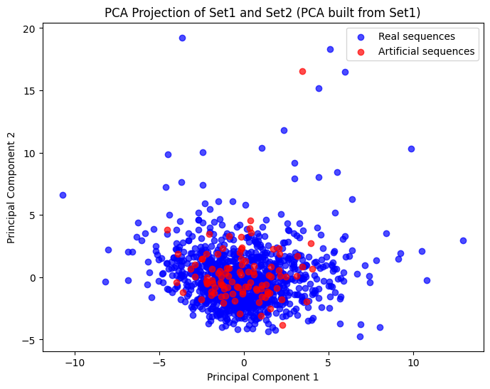
To visualize and compare real and generated DNA sequences in a continuous space, we can utilize Principal Component Analysis (PCA). PCA is a powerful dimensionality reduction technique that transforms high-dimensional data into a lower-dimensional space while preserving as much variability as possible. This allows us to visualize the similarities and differences between the sequences effectively.

def plot_pca_projection(set1: np.ndarray, set2: np.ndarray, title: str = "PCA Projection") -> None:
    """
    Fit PCA on set1 and project both set1 and set2 into the PCA space, then plot the results.

    Parameters:
    - set1 (np.ndarray): K-mer count matrix for the first set of sequences (used to fit PCA).
    - set2 (np.ndarray): K-mer count matrix for the second set of sequences (projected into PCA space).
    - title (str): Title of the plot.

    Returns:
    - None
    """
    # Fit PCA on set1 only
    pca = PCA(n_components=2)
    pca.fit(set1)

    # Project both set1 and set2 into the PCA space
    pca_set1 = pca.transform(set1)
    pca_set2 = pca.transform(set2)

    # Plot the first two principal components
    plt.figure(figsize=(8, 6))
    plt.scatter(
        pca_set1[:, 0],
        pca_set1[:, 1],
        color="blue",
        label="Real sequences",
        alpha=0.7,
    )
    plt.scatter(
        pca_set2[:, 0],
        pca_set2[:, 1],
        color="red",
        label="Artificial sequences",
        alpha=0.7,
    )

    # Add labels and legend
    plt.xlabel("Principal Component 1")
    plt.ylabel("Principal Component 2")
    plt.title(title)
    plt.legend()

    # Show the plot
    plt.show()


plot_pca_projection(real_seq_kmer_counts, artificial_seq_kmer_counts)

Hands On

For different temperature values (\(0.001\), \(0.01\), \(0.1\), \(0.5\), \(1.0\), \(1.5\)):

1. Generate synthetic DNA sequences
2. Observe the 5 first generated sequences
3. Generate the PCA plots
4. Compute the variance of k-mers counts between artificial sequences

Solution

def generate_synthetic_dna(
    model_name: str,
    max_length: int,
    num_sequences: int,
    temp: float,
    top_k: int = 50,
    repetition_penalty: float = 1.2,
) -> List[str]:
    """
    Generate synthetic DNA sequences using a pre-trained language model.
    
    Parameters:
    - model_name (str): Name or path of the pre-trained model.
    - max_length (int): Maximum length of each generated sequence.
    - num_sequences (int): Number of sequences to generate.
    - temp (float): Temperature value to control sequence variability.
    - top_k (int): Number of highest probability vocabulary tokens to consider. Default is 50.
    - repetition_penalty (float): Penalty for repeating the same token. Default is 1.2.
    
    Returns:
    - List[str]: List of generated DNA sequences.
    """
    # Initialize the sequence generation pipeline
    generator = pipeline("text-generation", model=model_name)
    # Generate synthetic DNA sequences
    synthetic_dna = generator(
       "",
       max_length=max_length,
       do_sample=True,
       top_k=top_k,
       temperature=temp,
       repetition_penalty=repetition_penalty,
       num_return_sequences=num_sequences,
       eos_token_id=0,
    )
    # Extract and clean the generated sequences
    artificial_sequences = [seq["generated_text"].replace(" ", "") for seq in synthetic_dna]
    return artificial_sequences


temperatures = [0.001, 0.01, 0.1, 0.5, 1.0, 1.5]
for temp in temperatures:
    art_sequences = generate_synthetic_dna(model_name, max_length,  num_sequences, temp)
    art_seq_kmer_counts, kmers = kmer_counts_matrix(art_sequences, k=k)
    plot_pca_projection(real_seq_kmer_counts, art_seq_kmer_counts)
    var = np.mean(np.var(art_seq_kmer_counts, axis=0))
    print(f"Variance for temperature of { temp }: { var }")

Question

1. How similar do the 5 first generated DNA sequences look like given the temperature?
2. What are the different values for the variance?
3. What can we conclude?

Solution

1. Lower the temperature, more similar the sequences.
2. The variance for the different temperatures are:
   • Variance \(=\) for temperature \(= 0.001\)
   • Variance \(=\) for temperature \(= 0.01\)
   • Variance \(=\) for temperature \(= 0.1\)
   • Variance \(=\) for temperature \(= 0.5\)
   • Variance \(=\) for temperature \(= 1\)
   • Variance \(=\) for temperature \(= 1.5\)
3. Higher the temperature, higher the variance, higher the variability.

Checking for Novelty in Generated DNA Sequences Using BLAST

After generating synthetic DNA sequences, it’s crucial to verify whether these sequences are truly novel or if they closely resemble existing sequences in biological databases. One effective method to accomplish this is by performing a BLAST (Basic Local Alignment Search Tool) search (Altschul et al. 1990). BLAST allows us to compare our generated sequences against a comprehensive database of known DNA sequences, helping us determine their uniqueness and potential biological relevance.

Let’s start with a synthetic DNA sequence generated with a low temperature setting. Low temperature settings reduce variability, making the generated sequences more similar to real sequences. This step helps ensure that the sequence is biologically plausible and likely to have counterparts in existing databases.

Hands On

1. Generate the synthetic DNA sequences with a temperature value of \(0.01\)
2. Get the first sequence
3. Make a Standard Nucleotide BLAST search of the first sequence

Solution

art_sequences = generate_synthetic_dna(model_name, max_length,  num_sequences, 0.01)
art_sequences[0]

Question

1. How many significant similarities have been found?
2. Have we generated new sequence?

Solution

1. The BLAST search do not return any significant match
2. When the BLAST search returns no significant matches, it suggests that the synthetic sequence is novel and does not closely resemble any known sequences. This outcome is particularly interesting because it indicates that the sequence generation process has produced something entirely new.

When generating sequences with low temperature, we observed limited variability among the sequences. This lack of variability can be useful for ensuring consistency but may limit the exploration of novel sequence spaces. To introduce more variability and potentially discover even more novel sequences, we can increase the temperature setting during sequence generation. Higher temperatures introduce greater randomness, leading to more diverse and potentially unique sequences.

Hands On

1. Generate the synthetic DNA sequences with a temperature value of \(1\)
2. Get the first sequence
3. Make a Standard Nucleotide BLAST search of the first sequence

Solution

art_sequences = generate_synthetic_dna(model_name, max_length,  num_sequences, 1)
art_sequences[0]

Question

1. How many significant similarities have been found?
2. Have we generated new sequence?

Solution

1. The BLAST search do not return any significant match
2. When the BLAST search returns no significant matches, it suggests that the synthetic sequence is novel and does not closely resemble any known sequences. This outcome is particularly interesting because it indicates that the sequence generation process has produced something entirely new.

Even if the generated sequences are novel, novelty alone does not guarantee functionality, so further analysis may be necessary to assess the potential applications of these sequences.

Exploring Synthetic Gene Generation

Having successfully generated and analyzed synthetic DNA sequences, the next intriguing question is: Can we extend this approach to generate entire synthetic genes? This endeavor requires producing longer sequences that mimic the complexity and functionality of natural genes. The mean length of yeast genes is several hundred bases. To effectively mimic natural genes, our synthetic sequences must match this length while maintaining biological plausibility. Generating longer sequences is not merely about increasing length; it’s about ensuring that these sequences contain the necessary genetic elements, such as promoters, coding regions, and regulatory sequences, that are essential for gene function.

To start, we generate 10 sequences with max_length = 400:

synthetic_dna = generate_synthetic_dna(model_name, 400, 10, 1)

Question

How long are the first 5 sequences?

Solution

Detecting Open Reading Frames (ORFs)

To determine if the generated sequences could contain genes, we examine them for the presence of key genetic elements, such as Open Reading Frames (ORFs).

An ORF is a portion of a DNA sequence that begins with a start codon (e.g., ATG) and ends with a stop codon (e.g., TAA, TAG, TGA). Identifying ORFs is essential for determining the potential functionality of synthetic DNA sequences, as ORFs can indicate whether a sequence could encode a protein.

To detect ORFs in sequences, we use orfipy_core:

def detect_orfs(
    sequence: str,
    minlen: int = 100,
    maxlen: int = 1000,
) -> List[Tuple[int, int, str, str]]:
    """
    Detect ORFs in a given DNA sequence.

    Parameters:
    - sequence (str): The DNA sequence to analyze.
    - minlen (int): Minimum length of ORFs to detect. Default is 100.
    - maxlen (int): Maximum length of ORFs to detect. Default is 1000.

    Returns:
    - List[Tuple[int, int, str, str]]: List of ORFs with start, stop positions, strand, and description.
    """
    orfs = []
    for start, stop, strand, description in orfipy_core.orfs(sequence, minlen=minlen, maxlen=maxlen):
        orfs.append((start, stop, strand, description))
        print(f"Start: {start}, Stop: {stop}, Strand: {strand}, Description: {description}")
    return orfs

Let’s extract the ORFs for the first DNA sequence:

seq = artificial_sequences[0]
orfs = detect_orfs(seq)

Question

How many ORFs have been detected for the first DNA sequence?

Solution

Extracting and Translating Detected Open Reading Frames (ORFs)

After detecting Open Reading Frames (ORFs) in our synthetic DNA sequences, the next step is to extract these ORFs and translate them into protein sequences. This process allows us to explore the potential protein products encoded by our synthetic genes, providing insights into their possible functions and biological roles.

To extract and translate the ORFs, we need to:

1. Extract the ORF Sequence: Using the start and stop positions identified by the detect_orfs function, we can extract the corresponding DNA sequence for each ORF. This sequence represents the potential protein-coding region within the synthetic DNA.
2. Translate the ORF: We can convert the DNA sequence of the ORF into its corresponding amino acid sequence. This step reveals the potential protein product encoded by the ORF.

def extract_and_translate_orf(
    sequence: str,
    orfs: List[Tuple[int, int, str, str]],
    orf_index: int = 0,
) -> str:
    """
    Extract an ORF from a DNA sequence and translate it into a protein sequence.

    Parameters:
    - sequence (str): The DNA sequence containing the ORF.
    - orfs (List[Tuple[int, int, str, str]]): List of detected ORFs with start, stop positions, strand, and description.
    - orf_index (int): Index of the ORF to extract and translate. Default is 0.

    Returns:
    - str: The translated protein sequence.
    """
    # Extract the ORF sequence using the start and stop positions
    start, stop, strand, description = orfs[orf_index]
    orf_sequence = sequence[start:stop]

    # Translate the ORF sequence into a protein sequence
    protein_sequence = str(Seq(orf_sequence).translate())

    return protein_sequence

For the first detected ORFs:

protein_seq = extract_and_translate_orf(seq, orfs)
print(f"Translated Protein Sequence: {protein_seq}")

After translating a synthetic DNA sequence into a protein sequence, the next crucial step is to analyze this sequence to uncover its potential biological function. This involves identifying known protein domains or motifs within the sequence that may indicate specific functions, such as binding sites or active regions. Verifying the biological plausibility of the translated sequence is essential, which can be achieved by comparing it to known protein sequences in databases like UniProt or GenBank using tools like Diamond and InterProScan. Additionally, examining the conservation of the sequence across different species can provide insights into its functional importance. If the sequence shows potential for biological function, it can serve as a starting point for further research, including structural modeling to predict its three-dimensional structure, functional assays to test its activity, and evolutionary studies to understand its origins and adaptations. This comprehensive analysis not only enhances our understanding of the generated sequences but also opens new avenues for scientific exploration and application in synthetic biology and genetic engineering.

Conclusion

Throughout this tutorial, we have explored the process of generating synthetic DNA sequences using a DNA Language Model (LLM), focusing on creating sequences that mimic the complexity and functionality of natural yeast genomes. We began by building a sequence generator, leveraging pre-trained models to produce synthetic DNA sequences with controlled variability.

We compared of these synthetic sequences to real yeast genomes, utilizing k-mer counts and Principal Component Analysis (PCA) to visualize and assess their similarities and differences. This comparative analysis provided valuable insights into how well our generated sequences aligned with natural counterparts, highlighting both the strengths and areas for improvement in our approach.

To ensure the novelty of our generated sequences, we conducted BLAST searches, confirming that many of our synthetic sequences were indeed unique and did not closely match existing sequences in biological databases. This step was crucial in validating the potential of our model to produce truly innovative DNA sequences.

Expanding our exploration, we delved into the realm of synthetic gene generation. By detecting Open Reading Frames (ORFs) within our synthetic sequences, we identified potential protein-coding regions that could be translated into amino acid sequences. This process allowed us to analyze the biological relevance and potential functions of the proteins encoded by our synthetic genes, opening avenues for further research and application.

In conclusion, this tutorial has demonstrated the power and potential of DNA LLMs in generating synthetic DNA sequences and exploring synthetic gene generation. By combining advanced computational techniques with biological insights, we have shown how to create novel sequences that not only mimic natural genomes but also offer new possibilities for synthetic biology and genetic engineering. As we continue to refine these methods, the future holds exciting prospects for innovation and discovery in the field of genomics.

You've Finished the Tutorial

Please also consider filling out the Feedback Form as well!

Key points

• DNA Language Models (LLMs) are effective tools for generating synthetic DNA sequences that mimic natural genomes, offering a powerful approach for exploring and innovating in synthetic biology.

• Adjusting parameters like temperature allows for controlling the variability of generated sequences, enabling the creation of both biologically plausible and novel DNA sequences.

• Comparing synthetic sequences with real genomes and using tools like BLAST to check for novelty are essential steps in validating the uniqueness and potential biological relevance of generated sequences.

• Detecting and translating Open Reading Frames (ORFs) in synthetic sequences provides insights into potential protein functions, paving the way for further research in genetic engineering and synthetic biology applications.

Frequently Asked Questions

• Topic FAQs
• Galaxy FAQs
• GTN Matrix Chat
• Galaxy Help Forum

References

1. Altschul, S. F., W. Gish, W. Miller, E. W. Myers, and D. J. Lipman, 1990 Basic local alignment search tool. Journal of molecular biology 215: 403–410. 10.1016/S0022-2836(05)80360-2
2. Peter, J., M. De Chiara, A. Friedrich, J.-X. Yue, D. Pflieger et al., 2018 Genome evolution across 1,011 Saccharomyces cerevisiae isolates. Nature 556: 339–344. 10.1038/s41586-018-0030-5

Feedback

Did you use this material as an instructor? Feel free to give us feedback on how it went.
Did you use this material as a learner or student? Click the form below to leave feedback.

Citing this Tutorial

1. Raphael Mourad, Bérénice Batut, Generating Artificial Yeast DNA Sequences using a DNA LLM (Galaxy Training Materials). https://training.galaxyproject.org/training-material/topics/statistics/tutorials/genomic-llm-sequence-generation/tutorial.html Online; accessed TODAY
2. Hiltemann, Saskia, Rasche, Helena et al., 2023 Galaxy Training: A Powerful Framework for Teaching! PLOS Computational Biology 10.1371/journal.pcbi.1010752
3. Batut et al., 2018 Community-Driven Data Analysis Training for Biology Cell Systems 10.1016/j.cels.2018.05.012

BibTeX

@misc{statistics-genomic-llm-sequence-generation,
author = "Raphael Mourad and Bérénice Batut",
	title = "Generating Artificial Yeast DNA Sequences using a DNA LLM (Galaxy Training Materials)",
	year = "",
	month = "",
	day = "",
	url = "\url{https://training.galaxyproject.org/training-material/topics/statistics/tutorials/genomic-llm-sequence-generation/tutorial.html}",
	note = "[Online; accessed TODAY]"
}
@article{Hiltemann_2023,
	doi = {10.1371/journal.pcbi.1010752},
	url = {https://doi.org/10.1371%2Fjournal.pcbi.1010752},
	year = 2023,
	month = {jan},
	publisher = {Public Library of Science ({PLoS})},
	volume = {19},
	number = {1},
	pages = {e1010752},
	author = {Saskia Hiltemann and Helena Rasche and Simon Gladman and Hans-Rudolf Hotz and Delphine Larivi{\`{e}}re and Daniel Blankenberg and Pratik D. Jagtap and Thomas Wollmann and Anthony Bretaudeau and Nadia Gou{\'{e}} and Timothy J. Griffin and Coline Royaux and Yvan Le Bras and Subina Mehta and Anna Syme and Frederik Coppens and Bert Droesbeke and Nicola Soranzo and Wendi Bacon and Fotis Psomopoulos and Crist{\'{o}}bal Gallardo-Alba and John Davis and Melanie Christine Föll and Matthias Fahrner and Maria A. Doyle and Beatriz Serrano-Solano and Anne Claire Fouilloux and Peter van Heusden and Wolfgang Maier and Dave Clements and Florian Heyl and Björn Grüning and B{\'{e}}r{\'{e}}nice Batut and},
	editor = {Francis Ouellette},
	title = {Galaxy Training: A powerful framework for teaching!},
	journal = {PLoS Comput Biol}
}

                   

Galaxy Administrators: Install the missing tools

You can use Ephemeris's shed-tools install command to install the tools used in this tutorial.

shed-tools install [-g GALAXY] [-a API_KEY] -t <(curl https://training.galaxyproject.org/training-material/api/topics/statistics/tutorials/genomic-llm-sequence-generation/tutorial.json | jq .admin_install_yaml -r)

Alternatively you can copy and paste the following YAML

---
install_tool_dependencies: true
install_repository_dependencies: true
install_resolver_dependencies: true
tools: []

Feedback

No feedback has been recieved yet for this training. Be the first one by filling in the feedback form.